Fuzzy cluster networks highlight the fuzzy relationships among clustered data points using an intuitive two-dimensional network display. A powerful application of this approach is the visualization of differences between cell lines on the basis of differential gene expression. To display fuzzy cluster networks, a network visualization tool needs to be installed on your computer. Below, a protocol is given that requires Cytoscape [Shannon et al., 2005].

New! AutoSOME fuzzy clustering can now be performed directly in Cytoscape using the clusterMaker plugin. For additional details, see the paper.

Protocol

*You may skip steps 1-3 and use the tutorial datasets provided below.

1) Import your input file into AutoSOME, set fields and adjust input (see the manual for instructions).

2) Select Fuzzy Cluster Networks and choose distance metric. (Note that only vertical data vectors are clustered (e.g. cell samples or time series of a microarray dataset)

3) Run AutoSOME

4) Launch Cytoscape

5) Within Cytoscape (All screenshots below taken from Cytoscape 2.6.0):

a. Go to File>Import>Network from Table (Text/MS Excel)...

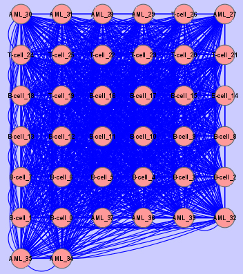
b. Go to Select File(s) and locate AutoSOME output file (4) containing all edges (see Files written to disk in the manual) or use the tutorial dataset.

c. Set Source Interaction to Column 1 and Target Interaction to Column 2. Finally, click on Column 3 in the data Preview window to activate it (it will turn blue).

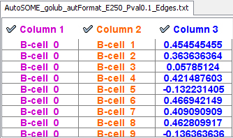
d. Select Import and then Close. A raw network will appear as a grid.

e. Go to File>Import>Attribute from Table (Text/MS Excel)...

f. Go to Select File(s) and locate AutoSOME output file (5) containing all nodes and attributes (see Files written to disk in the manual) or use the tutorial dataset.

g. Select Import.

h. Change global properties of the network:

i. In the Control Panel, select the VizMapperTM tab. Click in the Defaults window (shows a source and target pair with a blue background). A new window will appear. ii. Select the Global tab in the bottom right. iii. Change the background color to white. iv. Go back to the Node tab and change the NODE_BORDER_COLOR property to black and increase the NODE_LINE_WIDTH to 2. v. Select Apply

i. In the VizMapperTM tab:

j. Next to Node Label, click ID and select Column 3. All nodes should now be relabeled according to the original data labels. Minimize the Node Label property by selecting the minus icon.

k. Under Unused Properties find Edge Color and double-click it.

i. Select Column 3 as a value. ii. Select Continuous Mapper for Mapping Type. iii. Click on the black-to-white gradient next to Graphical View to launch a Gradient Editor. iv. There are two fixed triangles, one on each end, and two adjustable triangles. Double-click the two leftmost triangles and set their colors to pure red (255,0,0). Double-click the two rightmost triangles and set their colors to pure blue (0,0,255). Drag the leftmost adjustable triangle all the way to the left and likewise drag the rightmost triangle to the right until it stops.

l. Find Edge Line Width under Unused Properties and double-click it.

i. Select Column 3 as a value. ii. Select Continuous Mapper for Mapping Type. iii. Click on the graph next to the Graphical View property to launch the Continuous Editor. iv. Adjust the minimum and maximum values denoted by red squares (double-click on squares for precision, otherwise slide squares up or down). For example, set minimum to 0.5 and maximum to 20. Then, exit Continuous Editor.

m. Find Edge Opacity under Unused Properties and double-click it.

i. Select Column 3 as a value. ii. Select Continuous Mapper for Mapping Type. iii. Click on the graph next to the Graphical View property to launch the Continuous Editor. iv. Adjust the minimum and maximum values denoted by red squares (double-click on squares for precision, otherwise slide squares up or down). For example, set minimum to 0.5 and maximum to 60. Then, exit Continuous Editor.

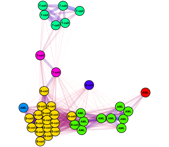
n. Finally, find Node Color under Unused Properties and double-click it.

i. Select Column 2 as a value. ii. Select Discrete Mapping for Mapping Type. iii. Right click on Discrete Mapping and go to Generate Discrete Values>Rainbow 1. All nodes are now colored according to cluster labels. Adjust colors as necessary.

o. Go to Layout in the main menu and select Settings

i. Choose Force-Directed Layout for Layout Algorithm ii. Under Edge Weight Settings, set The minimum edge weight to consider to -0.5, and set The maximum edge weight to consider to 0.5. Further, select Column 3 from The edge attribute that contains the weights. iii. Press Execute Layout to run the layout algorithm. iv. Although the network topology is generally preserved, different runs of the layout algorithm can yield slightly different results in terms of network rotation and local node placement. To increase the repulsion between neighboring nodes (for evenly spaced nodes within a cluster), increase Default Node Mass under Algorithm settings. Another layout algorithm that can yield comparable results is the Edge-weighted Spring Embedded algorithm. Before executing the layout, make sure the Edge Weight Settings are adjusted as in (ii) above. This layout algorithm can yield more evenly spaced nodes, but is less stable than Force-Directed Layout. Run a few times. v. Notice that all edges are slightly curved. To straighten edges, save and reopen the Cytoscape file. vi. At this point, make any desirable fine-grained changes to the Edge Color, Edge Line Width and Edge Opacity parameters to emphasize the fuzziness in the network.

p. To export the final network, go to File>Export>Network View as Graphics...

q. Select file format and save image!

r. To expedite this process for next time, start with your saved network. All visualization parameters will still be specified. Then, simply input your edge and node files and perform the layout. Note that for the Node Color property, it is important to assign colors again using the process given in step (n).